This code analyzes admissions data, focusing on predicting SAT Math scores using SAT Verbal scores and high school class size. The analysis employs linear regression models, including simple linear regression, multiple linear regression, correlation assessments, and visualizations to explore the relationships between these variables.
Here is the admissions data and you can download the script to run in R here
Load Necessary Libraries
library(foreign) # For reading .sav fileslibrary(ggplot2) # For visualization
Warning: package 'ggplot2' was built under R version 4.3.3
library(dplyr) # For data manipulation
Attaching package: 'dplyr'
The following objects are masked from 'package:stats':

    filter, lag
The following objects are masked from 'package:base':

    intersect, setdiff, setequal, union
library(gtsummary) # For creating regression tableslibrary(officer) # For exporting to Word
Warning: package 'officer' was built under R version 4.3.3
library(flextable) # For table formatting
Attaching package: 'flextable'
The following objects are masked from 'package:gtsummary':

    as_flextable, continuous_summary
Load and Inspect Data
admissions <-read.spss("data/admissions.sav", to.data.frame =TRUE)head(admissions) # Display first few rows
  row_number paiddeposit scholarship_yes_no Type_of_scholarship_offered Female
1          7           1                  0                                  0
2         12           0                  0                                  0
3         19           1                  0                                  0
4         23           1                  0                                  0
5         25           0                  0                                  0
6         28           0                  0                                  1
             Race HS_rank HS_class_size HS_Quintile HS_CODE
1 white               190           281        4/5   392835
2 white               111           223        3/5   393655
3 white               109           371        2/5    51830
4 Asian                88           266        2/5   390527
5 white                NA            NA              390870
6 white                59           382        1/5   392655
                  HS_NAME SAT_verbal ACT Honors_college_eligible
1 FRANKLIN_REGIONAL_SR_HI        560  NA                     no
2 CENTRAL_CATHOLIC_HIGH_S        600  NA                     no
3 WESTCHESTER_HIGH_SCHOOL        550  NA                     no
4 CEDAR_CLIFF_HIGH_SCHOOL        520  NA                     no
5 HOLY_GHOST_PREPARATORY         650  NA                     no
6 PENN_MANOR_HIGH_SCHOOL         460  20                     no
  distancefromPitt state Number_of_family_alumni father_alumni grand_alumni
1        14.228946    PA                       0             0            0
2         7.162134    PA                       0             0            0
3       232.363382    PA                       0             0            0
4       163.462296    PA                       0             0            0
5       261.534151    PA                       0             0            0
6       192.493359    PA                       0             0            0
  mother_alumni sibling_alumni step_parent_alumni other_family_alumni
1             0              0                  0                   0
2             0              0                  0                   0
3             0              0                  0                   0
4             0              0                  0                   0
5             0              0                  0                   0
6             0              0                  0                   0
  SAT_composite ACT_as_SAT Max_Test_Score Training from_PA
1          1180         NA           1180        0       1
2          1150         NA           1150        0       1
3          1190         NA           1190        0       1
4          1140         NA           1140        0       1
5          1200         NA           1200        0       1
6           940        950            950        0       1
               alumniYN SAT_math
1 Family is not an alum      620
2 Family is not an alum      550
3 Family is not an alum      640
4 Family is not an alum      620
5 Family is not an alum      550
6 Family is not an alum      480
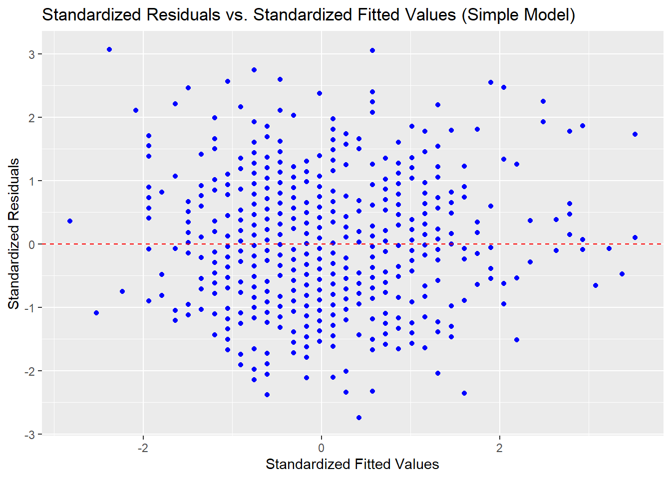
ggplot(admissions_clean, aes(x = std_fitted_simple, y = std_residuals_simple)) +geom_point(color ="blue") +geom_hline(yintercept =0, linetype ="dashed", color ="red") +labs(title ="Standardized Residuals vs. Standardized Fitted Values (Simple Model)",x ="Standardized Fitted Values", y ="Standardized Residuals")
Interpretation:
Residuals are fairly symmetrically distributed around zero, suggesting the linear model is appropriate.
No major patterns in residuals indicate homoscedasticity.
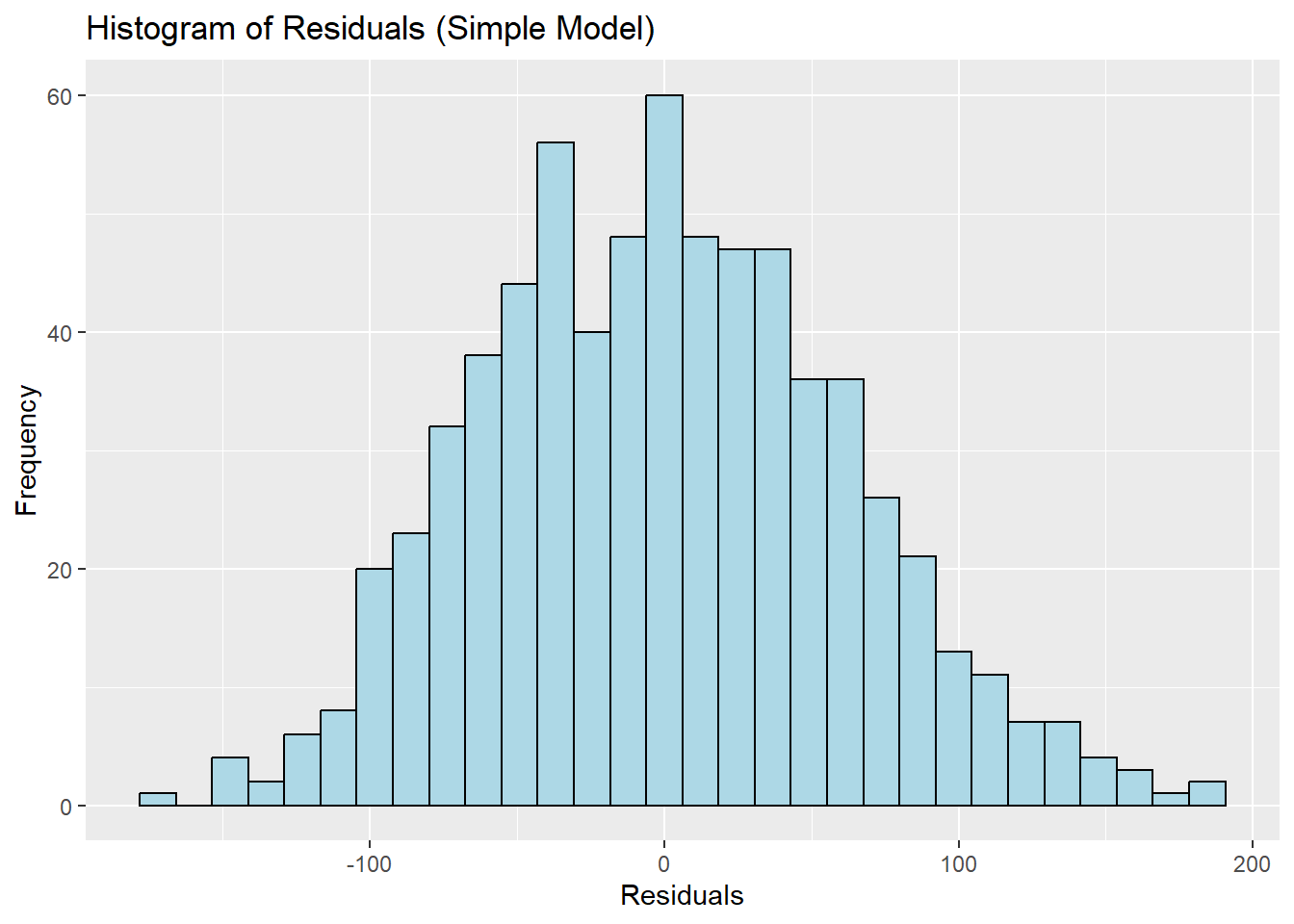
Histogram of Residuals
ggplot(admissions_clean, aes(x = residuals_simple)) +geom_histogram(bins =30, fill ="lightblue", color ="black") +labs(title ="Histogram of Residuals (Simple Model)", x ="Residuals", y ="Frequency")
Interpretation:
Residuals follow a normal-like distribution, supporting the assumption of normality.
Correlation Analysis
cor(admissions_clean[, c("SAT_math", "SAT_verbal", "fitted_simple", "residuals_simple")], use ="complete.obs")
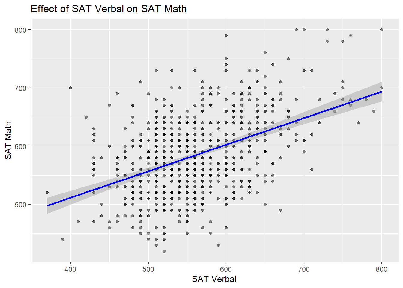
Strong positive correlation between SAT Math and SAT Verbal (r ≈ 0.45).
Fitted values highly correlate with SAT Verbal, confirming its predictive power.
Multiple Linear Regression: SAT Math ~ SAT Verbal + HS Class Size
multiple_model <-lm(SAT_math ~ SAT_verbal + HS_class_size, data = admissions_clean)summary(multiple_model)
Call:
lm(formula = SAT_math ~ SAT_verbal + HS_class_size, data = admissions_clean)

Residuals:
     Min       1Q   Median       3Q      Max
-165.924  -44.589   -1.418   40.825  197.261

Coefficients:
               Estimate Std. Error t value Pr(>|t|)
(Intercept)   314.14654   19.47735  16.129  < 2e-16 ***
SAT_verbal      0.44864    0.03401  13.192  < 2e-16 ***
HS_class_size   0.06030    0.01295   4.656 3.88e-06 ***
---
Signif. codes:  0 '***' 0.001 '**' 0.01 '*' 0.05 '.' 0.1 ' ' 1

Residual standard error: 60.52 on 688 degrees of freedom
Multiple R-squared:  0.2266,    Adjusted R-squared:  0.2244
F-statistic: 100.8 on 2 and 688 DF,  p-value: < 2.2e-16
Interpretation:
HS Class Size has a small but significant positive effect (Estimate = 0.06030, p < 0.001).
Explained variance increases to 22.4%, showing a slight improvement over the simple model.
Visualization of SAT Verbal Effect
ggplot(admissions_clean, aes(x = SAT_verbal, y = SAT_math)) +geom_point(alpha =0.5) +geom_smooth(method ="lm", col ="blue") +labs(title ="Effect of SAT Verbal on SAT Math", x ="SAT Verbal", y ="SAT Math")
`geom_smooth()` using formula = 'y ~ x'
Generate Regression Summary Table
mlr_table <- multiple_model %>%tbl_regression(label =list(SAT_verbal ="SAT Verbal Score", HS_class_size ="High School Class Size")) %>%modify_caption("Table 1: Multiple Linear Regression Results") %>%add_n()
Save Table to Word
mlr_flextable <-as_flex_table(mlr_table)doc <-read_docx()doc <-body_add_flextable(doc, value = mlr_flextable)print(doc, target ="MLR_Results.docx")
Conclusion
Key Findings:
SAT Verbal scores significantly predict SAT Math scores, explaining ~20% of the variance.
Adding HS Class Size improves the model slightly, raising the explained variance to 22.4%.
Both models suggest a linear relationship, with residuals showing normality and no major violations.
Implications:
Schools aiming to improve SAT Math scores may focus on strengthening verbal skills.
Class size appears to play a small but relevant role in performance.
Further research could explore additional predictors (e.g., socioeconomic factors, study habits).