Introduction
There is quite a bit of data wrangling that needs to be done before you can use the CDC's Places dataset. It is also nice to be able to have access to the data without having to download it onto your computer. Many open data websites allow you to connect to data in the repository through the Application Programming Interface, or API.
Here, I show you how this can be done using the Places dataset. The code connects to the data, reshapes, recodes and filters the data, and gets it ready for mapping, all in one fell swoop.
As you can see from the website the Places dataset has a lot of variables. I am going to only select the mental health variable to analyze.
I have never used this data in my own work yet, however, take a loot at this recent paper that did. The paper explores Neighborhood Walkability and Cardiovascular Risk in the United States. You could do something similar by merging this data with the national walkability index (see Datasets).
if(!"remotes" %in% installed.packages()) {
install.packages("remotes")
}
cran_pkgs = c(
"sf",
"tidygraph",
"igraph",
"osmdata",
"dplyr",
"tibble",
"ggplot2",
"units",
"tmap",
"rgrass7",
"link2GI",
"nabor"
)
remotes::install_cran(cran_pkgs)
library(sf)
library(tidygraph)
library(igraph)
library(dplyr)
library(tibble)
library(ggplot2)
library(units)
library(tmap)
library(osmdata)
library(rgrass7)
library(link2GI)
library(nabor)
library(RSocrata)
library(tidyr)
library(sf)
library(tigris)
library(tidyverse)
library(tidycensus)
library(stplanr)
library(censusapi)
# setwd("")
root.dir = "https://raw.githubusercontent.com/urbanSpatial/Public-Policy-Analytics-Landing/master/DATA/"
source("https://raw.githubusercontent.com/urbanSpatial/Public-Policy-Analytics-Landing/master/functions.r")
options(scipen=10000)
#https://datacatalog.cookcountyil.gov/api/odata/v4/cjeq-bs86
cdc_places <-
read.socrata("https://data.cdc.gov/resource/nw2y-v4gm.json?") %>%
#read.csv("C:/Users/barboza-salerno.1/Downloads/PLACES__Local_Data_for_Better_Health__Census_Tract_Data_2022_release.csv") %>%
dplyr::filter(stateabbr == 'OH' & countyname == "Franklin" & year == 2020) %>%
dplyr::mutate(x = gsub("[c()]", " ", geolocation.coordinates)) %>%
#trim(x) %>%
separate(x,into= c("X","Y"), sep=",") %>%
dplyr::select(
GEOID = locationname,
category = category,
measure = measure,
value = data_value,
lci = low_confidence_limit,
uci = high_confidence_limit,
pop = totalpopulation, X, Y
) %>%
dplyr::mutate(
X = as.numeric(as.character(X)),
Y = as.numeric(as.character(Y)),
value = as.numeric(as.character(value)),
lci = as.numeric(as.character(lci)),
uci = as.numeric(as.character(uci))
) %>%
pivot_wider(names_from = c(category:measure), values_from = c(value:uci)) %>%
dplyr::select(GEOID, `value_Health Status_Mental health not good for >=14 days among adults aged >=18 years` , X, Y) %>%
dplyr::rename(mental_health = `value_Health Status_Mental health not good for >=14 days among adults aged >=18 years`) %>%
st_as_sf(coords = c("X", "Y"), crs = 4326, agr = "constant") %>%
st_transform("+proj=longlat +datum=WGS84 +no_defs") -> cdc_places_sf
st_read("https://raw.githubusercontent.com/deldersveld/topojson/master/countries/us-states/OH-39-ohio-counties.json") %>%
filter(NAME == "Franklin") %>%
st_set_crs(4326) %>%
st_transform("+proj=longlat +datum=WGS84 +no_defs") -> ohio
border <- st_union(ohio)
#url = "https://edg.epa.gov/EPADataCommons/public/OA/WalkabilityIndex.zip"
library(crsuggest)
walkies <- st_read("I:/health/ohio/NationalWalkabilityI_Project1.shp") %>%
st_set_crs(4326) %>%
st_transform("+proj=longlat +ellps=GRS80 +towgs84=0,0,0,0,0,0,0 +no_defs")
rivers <- linear_water(state = "Ohio", "Franklin", class="sf")
water <- area_water(state = "Ohio", "Franklin", class = "sf")
rd <- roads(state = "Ohio", "Franklin", class = "sf") %>%
filter(RTTYP == "I")
ggplot() +
geom_sf(data = walkies, color = "white", size = 0.0725, aes(fill = NatWalkInd)) +
geom_sf_label(
data = ohio, aes(label = ""), size = 4, lineheight = 0.875,
label.padding = unit(0.05, "lines"), label.size = 0, fill = "white"
) +
scale_fill_viridis_c(
direction = -1, limits = c(0,20), name = "Walkability Index",
breaks = seq(0, 20, 3), labels = c("0 (Nigh impassable)", 3, 6, 9, 12, 15, "20 (Very walkable)")
) +
labs(
x = NULL, y = NULL,
title = "Walkability Index for Franklin County, Ohio",
caption = "Data source: EPA DataCommons Walkability Index"
) +
theme(plot.title = element_text(hjust = 0.5)) +
theme(legend.position = c(0.85, 0.25)) +
theme(legend.title = element_text( hjust = 0.5)) +
theme(legend.box.background = element_rect(color = "#2b2b2b", fill = "white")) + theme_void()
walkies_CT <- walkies %>%
unite("GEOID", STATEFP:TRACTCE, sep = "", remove = FALSE) %>%
dplyr::select(GEOID, NatWalkInd) %>%
group_by(GEOID) %>% summarize(NatWalkInd = mean(NatWalkInd))
walkies_CT <- walkies_CT %>% left_join(cdc_places)
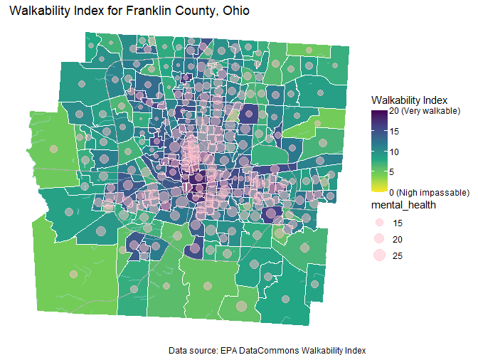
ggplot() +
geom_sf(data = walkies_CT, color = "white", size = 0.0725, aes(fill = NatWalkInd)) +
geom_sf(data = cdc_places_sf, color = "pink", aes(size = mental_health), alpha = 5/10) +
#geom_sf(data = walkies_CT, color = "white", size = 0.0725, aes(fill = value_BINGE_RISKBEH)) +
geom_sf(data = rd, color = "#999999", size = 2, alpha = 1/10) +
geom_sf(data = rd, color = "white", size = 1, alpha = 1/5) +
geom_sf(data = rd, color = "#aaaaaa", size = 1/2, alpha = 1/2) +
geom_sf(data = rivers, color = "lightblue", size = 1/2, alpha = 1/2) +
geom_sf_label(
data = ohio, aes(label = ""), size = 4, lineheight = 0.875,
label.padding = unit(0.05, "lines"), label.size = 0, fill = "white"
) +
scale_fill_viridis_c(
direction = -1, limits = c(0,20), name = "Walkability Index",
breaks = seq(0, 20, 5), labels = c("0 (Nigh impassable)", 5, 10, 15, "20 (Very walkable)")
) +
labs(
x = NULL, y = NULL,
title = "Walkability Index for Franklin County, Ohio",
caption = "Data source: EPA DataCommons Walkability Index"
) +
theme(plot.title = element_text(hjust = 0.5)) +
theme(legend.position = c(0.85, 0.25)) +
theme(legend.title = element_text( hjust = 0.5)) +
theme(legend.box.background = element_rect(color = "#2b2b2b", fill = "white")) + theme_void()
This code produces the plot of mental health and walkability. As an exercise, you should change the mental health variable to obesity and explore the spatial relations.