What can I do with this data? The experimental Household Pulse Survey is designed to quickly and efficiently deploy data collected on how people’s lives have been impacted by the coronavirus pandemic. Data collection for Phase 3.9 of the Household Pulse Survey started on June 7, 2023 and is scheduled to continue until August 7, 2023. Phase 3.9 will continue with a two-weeks on, two-weeks off collection and dissemination approach. The links below will take you to the downloadable tables in XLSX for each release period.
Prior data collections phases
- Phase 1: April 23, 2020 - July 21, 2020
- Phase 2: August 19, 2020 - October 26, 2020
- Phase 3: October 28, 2020 - March 29, 2021
- Phase 3.1: April 14, 2021 - July 5, 2021
- Phase 3.2: July 21, 2021 – October 11, 2021
- Phase 3.3: December 1, 2021 – February 7, 2022
- Phase 3.4: March 2, 2022 – May 9, 2022
- Phase 3.5: June 1, 2022 – August 8, 2022
- Phase 3.6: September 14, 2022 – November 14, 2022
- Phase 3.7: December 9, 2022 – February 13, 2023
- Phase 3.8: March 1, 2023 – May 8, 2023
Note: Phase 1 of the Household Pulse Survey was collected and disseminated on a weekly basis. All later phases of the survey have used two-week collection and dissemination periods. Despite going to a two-week collection period, the Household Pulse Survey continues to call these collection periods "weeks" to maintain continuity. Phases 3.3 and later maintain the two-week collection periods but shifted to a two-weeks on, two-weeks off collection approach. As a result there will continue to be three data collection and dissemination cycles instead of six for Phase 3.8.
I created a script to automatically download and begin to analyze this data. I was interested in debt during the pandemic, however there are a lot of variables that are interesting including depressive symptoms and health behaviors. This script downloads all of the pulse datafiles for the state of OHIO for the years that the data are available. It also cleans and merges a few datasets and makes a chart.
> You can do this by hand if you have an extra two years or so <
library(qdapRegex)
library(gdata)
library(rvest)
library(plyr)
library(ggthemes)
library(dplyr)
library(ggplot2)
options(timeout=120)
DIR <- "C:/Users/barboza-salerno.1/OneDrive - The Ohio State University/Documents/pulse"
#easiest way to get tags of interest
get_refs_on_page <- function(page){
refs = lapply(tryCatch({readLines(page)}, error=function(cond){return(NA)},warning=function(cond){return(NA)}), function(x) {y=rm_between(x , "href=\"", "\"", extract=TRUE)[[1]]})
refs=unlist(refs)
refs = refs[!is.na(refs)]
return(refs)
}
#this is the census bureau's pulse survey website
page <- "https://www.census.gov/programs-surveys/household-pulse-survey/datasets.html"
a <- readLines(page)
refs_1 = get_refs_on_page(page)
#find lines associated with CSV zip files
loc.zip <- grep('_PUF_CSV.zip', refs_1)
for (i in 21:length(refs_1[loc.zip])) {
refs_1[loc.zip][i] <- paste0("https:", trim(refs_1[loc.zip][i]))
}
download.files <- function(url, destfile = basename(url), ...){
for(i in 1:length(url)){
download.file(url[i], destfile[i], ...)
}
}
# iterate and download
download.files(noquote(refs_1[loc.zip]), basename(refs_1[loc.zip]))
#################################### Unzip and read files
# get all the zip files
zipF <- list.files(path = DIR, pattern = ".zip", full.names = TRUE)
# unzip all your files
ldply(.data = zipF, .fun = unzip, exdir = DIR)
# to illustrate we can read in one file "C:\Users\giaba\Documents\Projects\Debt\pulse\pulse2022_data.dictionary_CSV_45.xlsx"
df_w01 <- read.csv("C:/Users/barboza-salerno.1/OneDrive - The Ohio State University/Documents/pulse/pulse2020_puf_01.csv")
df_w45 <- read.csv("C:/Users/barboza-salerno.1/OneDrive - The Ohio State University/Documents/pulse/pulse2022_puf_45.csv")
df_w59 <- read.csv("C:/Users/barboza-salerno.1/OneDrive - The Ohio State University/Documents/pulse/pulse2023_puf_59.csv")
# let's pull out data from California
df_w01 <- df_w01 %>% dplyr::filter(EST_ST == "39" )
df_w45 <- df_w45 %>% dplyr::filter(EST_ST == "39" )
df_w59 <- df_w59 %>% dplyr::filter(EST_ST == "39" )
df_w01 <- df_w01 %>% dplyr::select(MORTCONF, INCOME) %>% mutate(week = "Week 1")
df_w45 <- df_w45 %>% dplyr::select(MORTCONF, INCOME) %>% mutate(week = "Week 45")
df_co <- rbind(df_w01, df_w45)
df_w01 <- read.csv("C:/Users/barboza-salerno.1/OneDrive - The Ohio State University/Documents/pulse/pulse2020_puf_01.csv")
df_w01 <- df_w01 %>% dplyr::filter(EST_ST == "39" )
df_w01_1 <- df_w01 %>% dplyr::select(WORRY, INTEREST, DOWN) %>% mutate(week = "Week 1")
df_w59 <- df_w59 %>% dplyr::select(WORRY, INTEREST, DOWN) %>% dplyr::mutate(week = "Week 59")
df_co1 <- rbind(df_w01_1, df_w59)
df_co1[df_co1==-88] <- NA
df_co1[df_co1==-99] <- NA
df_co1$dep_sym <- df_co1$WORRY +df_co1$INTEREST +df_co1$DOWN
df_co1 %>% group_by(week) %>% summarise_each(funs(mean(., na.rm = TRUE)))
df_co[df_co==-88] <- NA
df_co$INCOME[df_co$INCOME==-99] <- NA
df_co$MORTCONF[df_co$MORTCONF==-99] <- NA
table(df_co$MORTCONF)
table(df_co$INCOME)
summary(df_co$INCOME)
df_co$Inc_cat <- cut(df_co$INCOME, breaks=c( 0, 3.000, 6.000, Inf), labels=c("Low Income", "Middle Income", "High Income"))
df_co <- df_co %>% mutate(MORTCONF=recode(MORTCONF,
`1`="Not at all/Slightly",
`2`="Not at all/Slightly",
`3`="Moderately",
`4`="Highly",
))
table(df_co$Inc_cat, df_co$MORTCONF)
toPlot<-df_co%>% filter(!is.na(MORTCONF) & !is.na(Inc_cat)) %>%
dplyr::group_by(Inc_cat, MORTCONF, week) %>%
dplyr::summarise(n = n()) %>%
dplyr::group_by(MORTCONF, week) %>%
dplyr::mutate(prop = n/sum(n))
ggplot(data = subset(toPlot, !is.na(MORTCONF) & !is.na(Inc_cat) ), aes(Inc_cat , prop, fill = MORTCONF, na.rm = TRUE)) +
geom_col () +
facet_grid(~week+MORTCONF)+scale_fill_manual(values = c("blue","green", "red")) +
labs(x = "Confidence in Ability to Pay Mortgage", y = "Proportion of Respondents", title = "Income and Mortgage Dept",
subtitle = "How confident are you that your household will be able to pay your next rent or mortgage payment on time?\nWeeks 1 and Week 45", fill = 'Income Categories')+
scale_color_fivethirtyeight() +
theme_fivethirtyeight()
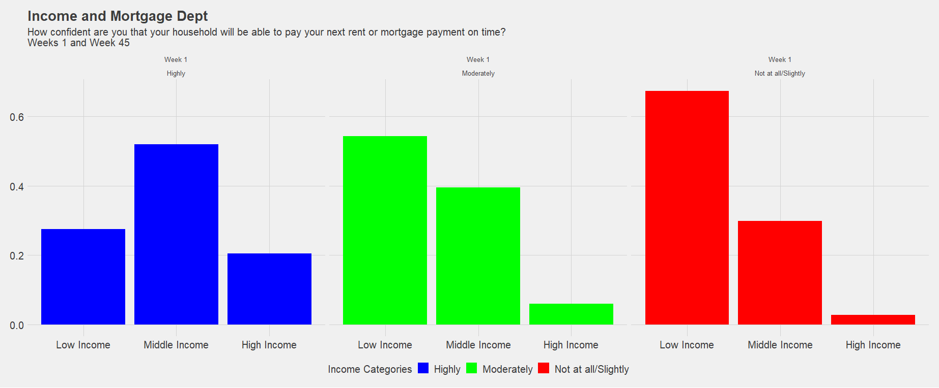
Fig 1. Income categories and mortgage debt for Week 1 of the COVID-19 pandemic.
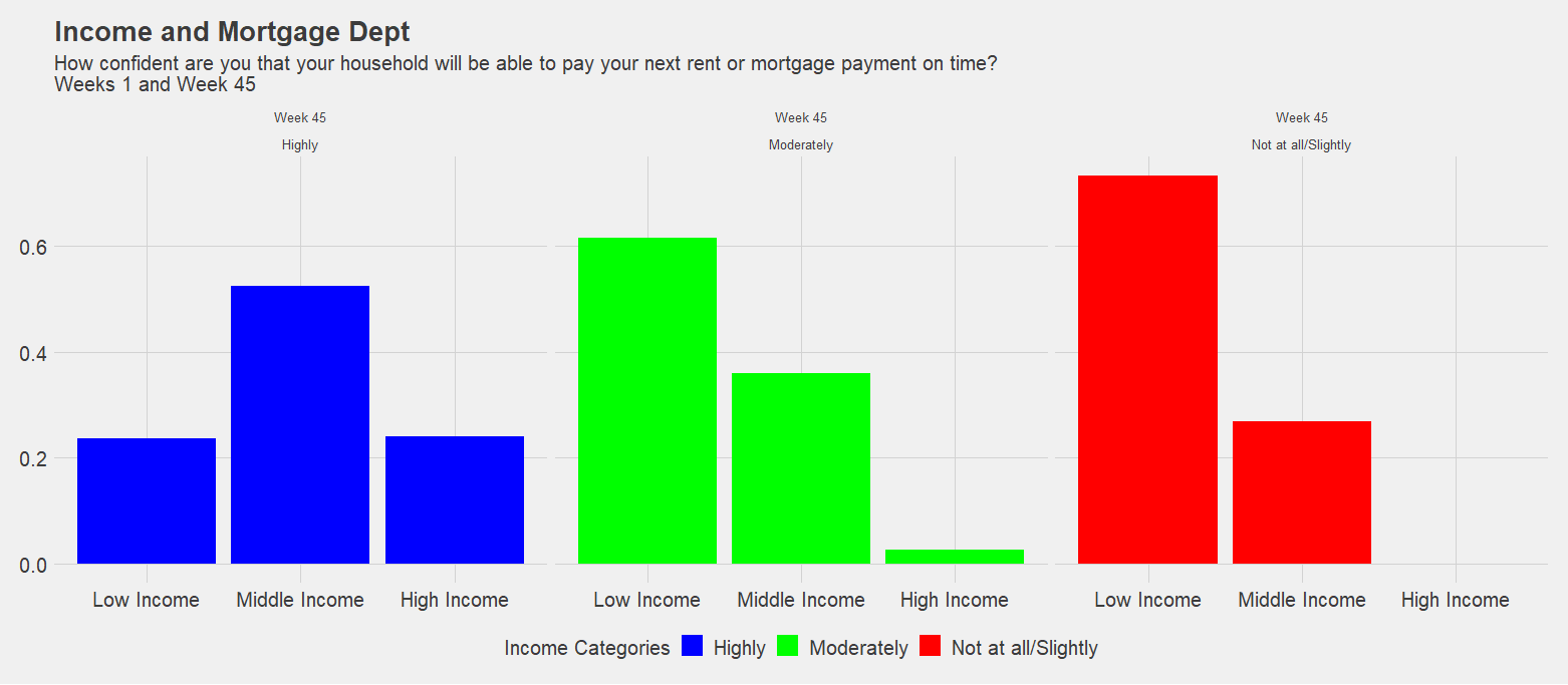
Fig 2. Income categories and mortgage debt for Week 45 of the COVID-19 pandemic.